sfmflex-release
Public code for "Visualizing Spectral Bundle Adjustment Uncertainty", 3DV 2020.
This project is maintained by wilsonkl
Visualizing Spectral Bundle Adjustment Uncertainty
Kyle Wilson and Scott Wehrwein, 3DV 2020. (Poster, 9MB pdf)
You can find online interactive versions of our visualizations here.
Abstract
Bundle adjustment is the gold standard for refining solutions to geometric computer vision problems. This paper develops an uncertainty visualization technique for bundle adjustment solutions to Structure from Motion problems.
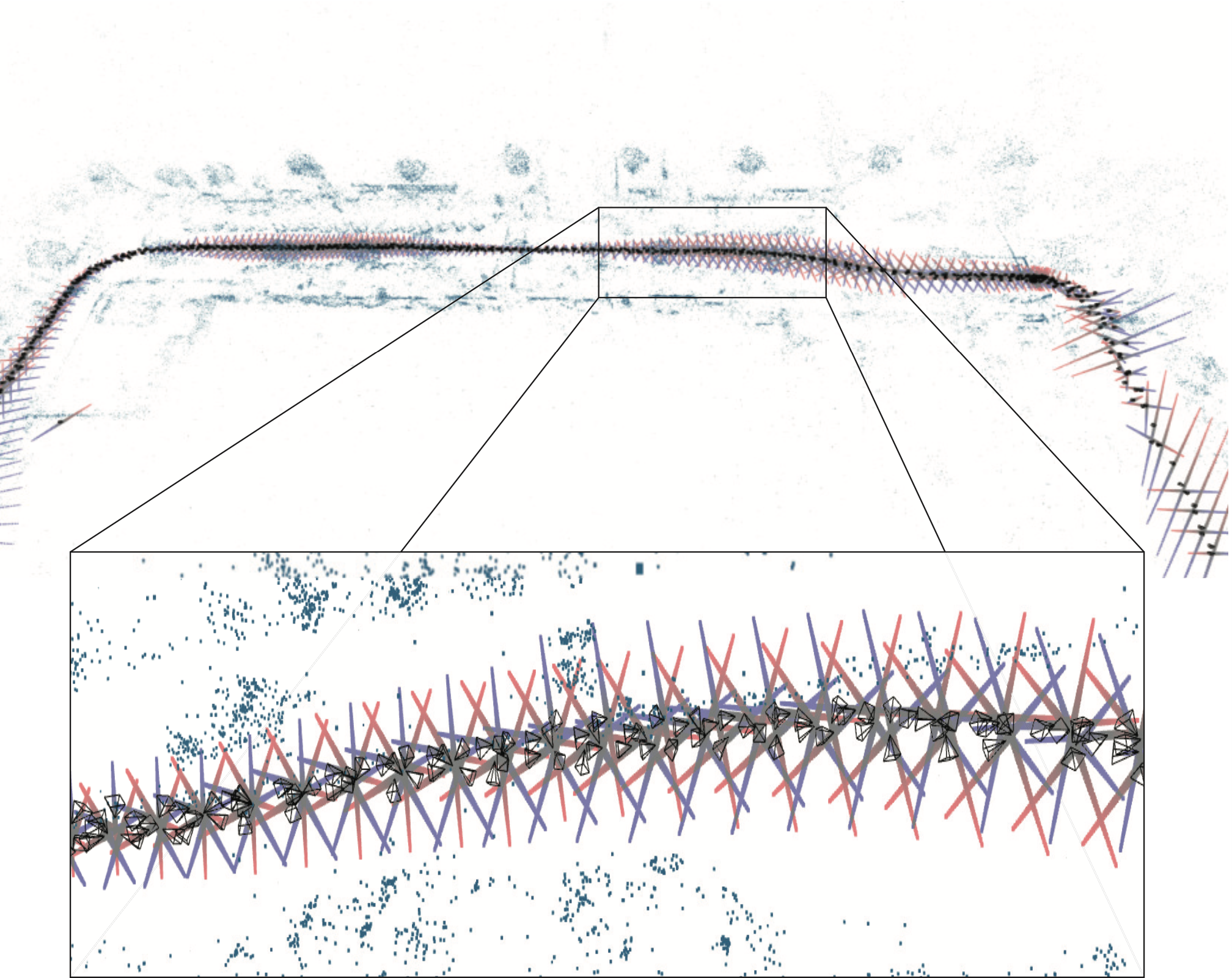
Propagating uncertainty through an optimization–from measurement uncertainties to uncertainties in the resulting parameter estimates–is well understood. However, the calculations involved fail numerically for real problems. Often we cope by considering only individual variances, but this ignores the important mutual dependencies between parameters. The dominant modes of uncertainty in most models are large motions involving nearly all parameters at once. These frequently look like flexions, stretchings, and bendings in the overall scene structure.
In this paper we present a numerically tractable method for computing dominant eigenvectors of the covariance of a Bundle Adjustment solution. We pay careful attention to the mismatched scales of rotational and translational parameters. Finally, we animate this spectral information. The resulting interactive visualizations (included in the supplemental) give insight into the quality and failure modes of a model. We hope that this work is a step towards broader uncertainty-aware computation for Structure from Motion.
Overview
This repository contains:
- Interactive web visualizations that accompany our 3DV20 paper
- The research code that produces these visualizations
Visualizations
Live versions of the visualizations in our paper can be accessed by the links below:
These visualizations are included in the supplemental to our paper and in this repository. Please see the supplemental commentary for interpretive remarks.
Demo controls
| Action | Control |
|---|---|
| Toggle scene point visibility | p |
| Rotate the model | click + drag |
| Translate the model | altclick + drag |
| Next/previous eigenvector | j/k |
| Increase/decrease translation scale | h/l |
| Increase/decrease rotation scale | g/; |
| Help popup | ? |
How to run the demos locally
Please clone this repository. There are HTML files for each scene in the visualizations directory. Open these in any web browser (tested: Firefox, Chrome, Safari).
Research Code
The code pipeline works as follows:
- Given a Structure from Motion problem instance in the format of Bundle Adjustment in the Large or Bundler
- Run a stock bundle adjuster to guarantee that we are at a local minimum (otherwise the Gauss-Newton approximation will be terrible!)
- Extract the problem parameters and its derivatives and save them out to an HDF5 file.
- Read the HDF5 file, compute eigenvectors, and save the eigenvectors and scene parameters to a JSON file.
- Load the JSON file and display an interactive visualization.
The preprocessing stages are based on ceres-solver and its included bundle adjuster. This is in C++. The eigenvector computations are performed in Julia, and the final interactive visualization is based on ThreeJS in Javascript.
Setup and Building
The C++ targets depend on Eigen, GFlags, Glog, and hdf5. They also require ceres-solver, which should be built from source. Be sure to build ceres with suite-sparse.
For convenience on Ubuntu: apt-get install libeigen3-dev libgoogle-glog-dev libgflags-dev libhdf5-dev
Also, download the header-only library HighFive:
# from the sfmflex-release/code/ directory
mkdir lib && cd lib
git clone https://github.com/BlueBrain/HighFive.git
To build the C++ targets:
# from the sfmflex-release/code/ directory
mkdir build
cd build
cmake ..
make
The Julia code also has many dependencies. Install all of these by running julia deps.jl from the sfmflex-release/code/ directory.
Datasets
We have run our method on two datasets:
- Bundle Adjustment in the Large problems
- 1DSfM problems
A script is provided below to scrape and download all of the BAL problems. The 1DSfM problems are available as a single download from the 1DSfM project page.
Scripts and bins
Run all of these scripts from the sfmflex-release/code/ directory.
Pipeline scripts: These script don’t take CLI options—edit their options in the file.
julia scripts/generate_json_for_vis.jl: pipeline script to take a BAL-formatted SfM problem instance and produce a json file suitable for running in the visualizer.julia scripts/run_1dsfm_datasets.jl: run all the 1dsfm problems through the pipeline and generate vis files.
Dataset scripts: These are useful for downloading problem instances and converting between file formats.
julia scripts/download_bal.jl: scape, download, and decompress all of the BAL datasets. Store them atsfmflex-release/code/dataset/bal/.julia scripts/run_ba_on_bal.jl: run a bundle adjuster on all BAL problems found atsfmflex-release/code/dataset/bal/. This takes a long time.julia scripts/bundle2bal.jl <bundle_file> <bal_file>: convert problem formats from a bundler.outproblem instace to a BAL problem instance.
Preprocessing scripts: These scripts are used within the pipeline scripts.
build/bin/compute_jacobian <bal_problem> <jac_file>: compute the Jacobian of a bundle adjustment problem.build/bin/bundle_adjuster: an all-purpose bundle adjuster, lightly tweaked from the ceres-solver example. There are many command line options.
Viewing the Visualizations
To view the interactive visualizations, first run one of the pipeline scripts above to get a json file containing the scene parameters and the computed covariance eigenvectors. Then edit sfmflex-release/code/vis/vis_supp.html (line 43) to include that json file. (The include path is relative to the vis_supp.html file.) Now open vis_supp.html in any web browser.
File Formats
BAL problems The Bundle Adjustment in the Large datasets use the same camera model as Bundler. See the BAL project page for details. Notice that unlike Bundler, the 2D coordinate system has its origin at the image center.
The BAL (and Bundler) cameras map 3D world coordinates X into 3D camera-centered coordinates Y via Y = R*X + t.
The camera parameters are ordered as:
r1, r2, r3, t1, t2, t3, f, k1, k2
Jacobian text files (Some older code stores Jacobians in text files. This has been mostly replaced by HDF5 files for performance.)
The first line of each file gives dimensions:
num_cameras num_points num_observations
The remainder of the file gives the Jacobian in (i, j, value) sparse triplets.
The Jacobian has dimensions (2*num_residuals) x (9*num_cameras + 3*num_points). The cameras are ordered first, and then the points, using the indexing of the source problem.
For now, no robust loss is applied when computing the Jacobian. This seems like an oversight that we’ll have to come back to.
Bundle Adjustment problem HDF5 files
See jl/JacobianUtils.jl:readproblem() for details about how a Bundle Adjustment problem is stored in an HDF5 file. Both a solution and its Jacobian, along with some other metadata, are all stored in binary format.
Visualization JSON files
We use json files to hold a scene + eigenvectors description in a way that is easy to read into our WebGL visualizer. See scripts/generate_json_for_vis.jl for a sample script that takes a BAL problem and outputs a vis json.
These json files are dictionaries at the base level containing the following fields:
num_camerasnum_pointscamera_parameters: a9*num_camerasvector ofdoubles. Parameter block order matches BAL:r1 r2 r3 t1 t2 t3 f k1 k2. The camera rotation matrixRis given by its angle-axis representationr1 r2 r3. Notice that camera centers are nott1 t2 t3but ratherC=-R'*t.point_parameters: a3*num_pointsvector ofdoubles. This is the 3D coordinates of every point in the scene.eigenvectors: a list of eigenvectors. The first eigenvector corresponds to the direction of highest variance, with the vectors ordered in descending order. Each eigenvector is a6*num_camerasvector ofdoubleswith parameters blocks ordered asr1 r2 r3 t1 t2 t3.
To make it easy to read into JavaScript, the base level dictionary has a name:
sample_scene = {...}
(yes, this is hacky…)